Chapter 5 Jupyter Notebook ecosystem

5.1 Language support: kernels

The Jupyter system supports over 100 programming languages (called “kernels” in the Jupyter ecosystem) including Python, Java, R, Julia, Matlab, Octave, Scheme, Processing, Scala, and many more. Out of the box, Jupyter will only run the IPython kernel, but additional kernels may be installed. Language support continues to be added by the open source community and the best source for an up-to-date list is the wiki page maintained by the project: https://github.com/jupyter/jupyter/wiki/Jupyter-kernels. These projects are developed and maintained by the open source community and exist in various levels of support. Some kernels may be supported by a vast number of active (and even paid) developers, while others may be a single person’s pet project. When trying out a new kernel, we suggest exploring a kernel’s community of users and documentation to see if it has an appropriate level of support for your (and your students’) use.

Jupyter’s kernel flexibility allows instructors to pick the right language for a particular context. For example instructors may use Python to teach programming, while switching to R to teach statistics, and then perhaps Scala to teach big-data processing. Regardless of the language chosen, the Jupyter interface remains the same. Thus, some cognitive load can be lessened when using multiple languages within or across courses (e.g., the user interface stays the same between the student’s Digital Humanities and Biology courses). Students often appreciate consistent use of the same language within a course, however.

5.2 Using Jupyter notebooks

When using Jupyter notebooks on the data projector or large screen monitor in the classroom, we recommend giving the students specific instructions on the meaning of the user interface of the notebook. It is not exactly intuitive.

The first and most salient component of the notebook is the cell. Indeed, the entire contents of a notebook is composed of only cells. These cells can take one of two forms: text or code. We will descibe the authoring of a notebook in the following section; however, here we identify some of the subtle, yet important components of a code cell.

Code cells are composed of three areas: the input area, the display area, and the output area. The input area is identified by the In []: prompt to the left of the cell. Between the brackets of the In prompt can be one of three items: a number, an asterisk, or a blank. A number indicates that this cell has been executed and the value of the number indicates the order of execution. For example, normally, after you execute the first cell after opening a notebook, its prompt will read In [1]:.

Pro Tip

When teaching with notebooks, you often will want to refer to a cell my name. You could refer to a cell by its input prompt number. However, keep in mind that this number will change if you excecute the cell again, or that students may have different numbers if they, too, are executing their own copy of the notebook. A better way of referring to a cell may be to refer to the text right above the cell as that won’t change while you execute cells. For referring to lines of code, see the following section on Tips and Tricks.

Before executing a cell, the input prompt number area will be blank. Therefore, you can tell at a glance that that cell has not been executed yet. It may also be the case that if an input prompt does have a number in it, then the cell has been run in the past. However, the cell may not have been run during this session, and thus the output may be showing old results. We recommend running from the menu: Cell, All outputs, Clear at the beginning of a presentation. That initializes all cell inputs to the blank state.

During the execution of a cell, the input prompt will contain an asterisk. If it seems that too much time has passed and you still see In [*]: your code may be in an infinite loop, or you have lost communication with the kernel. You may have to interrupt or restart the kernel. This is discussed below.

Finally, it is important to keep separate the display and output areas below the input cell. The difference between these two areas is subtle and confusing, but is very important in some instances. The display area is reserved for any item that code has produced for viewing. That includes simple text (i.e., print("hello, world")) or figures from a plot. The output area is reserved for items that the cell “returns.” This is why in many notebooks you may see a variable assignment followed immediately by the variable, like this:

In this example, you wouldn’t actually see the value computed unless you print it to the display area, or return the value. Here, we return it as the last value of the cell.

Keep in mind that the bottom portion of the notebook on the screen or monitor may not be visible to students in the back of the room. Make sure that the font size is large enough, and that you don’t go too fast when demonstrating code that students don’t have access to. We also recommend that you hide the Jupyter toolbar and header to get more room for the actual notebook (select Toggle Header and Toggle View under the Jupyter View menu).

5.3 Authoring Jupyter notebooks

Before embarking on writing notebooks for your course, we recommend that you look around on the internet for related courses. A similar course for which an instructor has already generated notebooks could exist for you to use or adapt for your course. Notebook authors often are happy to collaborate on open source educational resources or have their resources be used by other instructors. The following sections focus on Python simply because it is currently the language with the largest Jupyter feature support.

5.3.1 Accessing documentation in the notebook

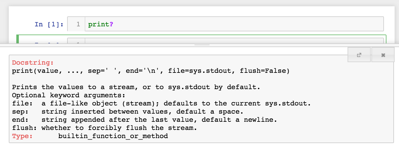
One of the best features of quality libraries is their documentation, which students and other users will likely consult regularly. From a notebook cell, the TAB key autocompletes (or gives completion tips) and SHIFT-TAB brings up full documentation. Similarly, using a question-mark after a method or function will bring up the documentation after the cell is run, as shown in Figure 5.1.

A question mark used after a method or function brings up the documentation after executing the cell.

A question mark used after a method or function brings up the documentation after executing the cell.

Using this feature in class during live coding or while explaining how code works helps make students comfortable of working effectively with libraries.

5.3.2 Widgets

Widgets provide the opportunity for learners and instructors to interact with code outputs, such as charts and tables. Widgets are “mini” Graphical User Interfaces (GUI) that give the notebook user access to slide bars, toggle buttons, and text-boxes. They can be used in conjunction with code, allowing a change of mindset from programming as a primary goal to exploring a model or computation as the primary goal. Alternatively, the code can be hidden and the widgets used to create a notebook “app” that might connect input parameters with a simulation and a plot.

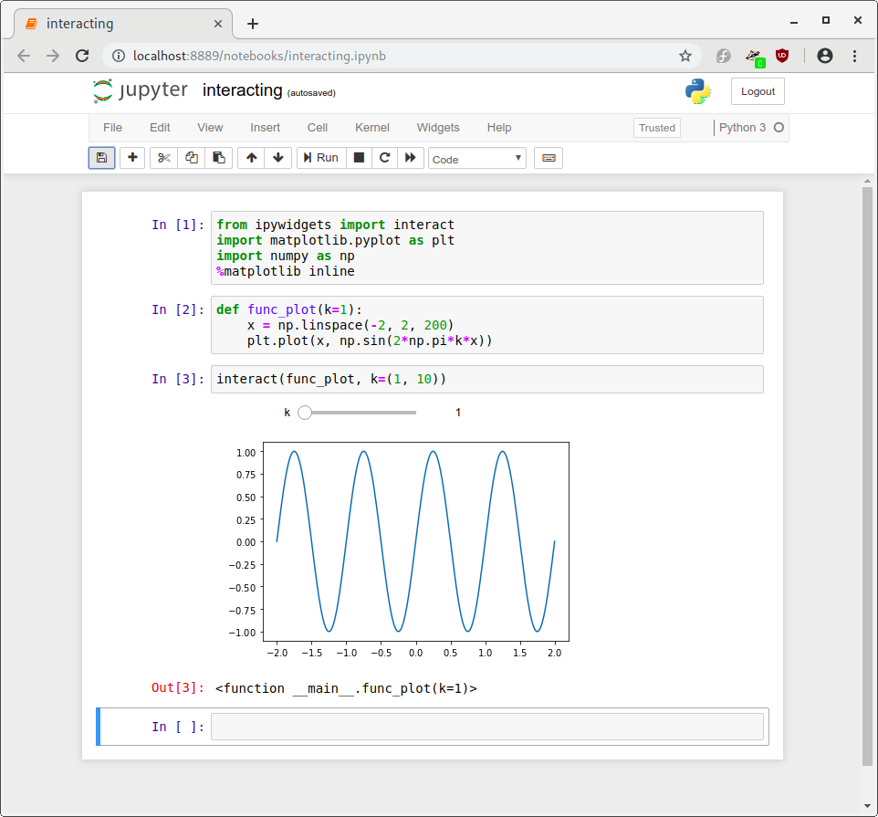
Currently, only a small subset of kernels have widget functionality. The reference implementation of widgets are the Jupyter-Python widgets (https://ipywidgets.rtfd.io). It includes widget components to generate and display sliders, progress bars, text boxes, check boxes, toggle buttons, etc. Many popular visualization tools, such as Matplotlib, Plotly, leaflet.js, three.js, have Jupyter-Python widget implementations. The documentation contains an up-to-date list of all of the widgets and their variations. The interact method allows you to wrap a function, which might be a simple computation or a complex simulation that produces a plot, and provides widgets for each of the inputs to the function. Figure 5.2 shows a simple example of a sinusoid plot whose frequency is controlled by a slide-bar. Another kernel that has some widget functionality is C++ (https://github.com/QUantStack/xwidgets).

Here, a slider allows the user to interactively change the variable k in our function as we plot it.

Here, a slider allows the user to interactively change the variable k in our function as we plot it.

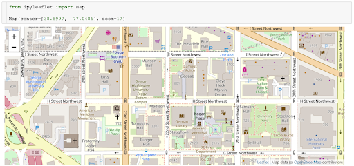
In addition to the IPywidgets library, the ipyleaflet library (https://ipyleaflet.rtfd.io) displays an interactive map in a notebook.

Example

from ipyleaflet import Map
Map(center=[34.6252978589571, -77.34580993652344], zoom=10)
Interactive map widget with ipyleafletalt_text.

Interactive map widget with ipyleafletalt_text.

For the ambitions reader, there are resources available for you to write your your own custom widgets. The widget cookie cutter project (https://ipywidgets.rtfd.io) is a good place to start.

5.3.3 Magics

Magics are meta-commands that only function within Jupyter and allow a user to access language/kernel-specific features. For instance, the IPython kernel provides a number of magics that can be useful while developing Jupyter notebooks using Python as the primary language. These are documented and we will only call out a few of these here. Many other magics are available for different kernels but they are specific to Jupyter so may not be usable in a stand-alone script in that language outside of Jupyter. In some instances, you may want to use magics sparingly to avoid obfuscating these meta-commands with the actual commands in the language you are teaching. Magics always begin with either a single % for single-line commands or with %% for applying a command to an entire cell. Some magics can be used with single or double %, but some cannot.

Examples

  • Matplotlib is a common choice for visualization. In Jupyter, the magic %matplotlib allows the resulting figures to be displayed in the notebook: %matplotlib inline produces static images embedded in the notebook, and %matplotlib notebook produces interactive images (with zooming, panning, etc.).

  • The %run magic allows running external scripts (and other notebooks), captures output and displays it in the notebook, e.g., %run my_script.py. The %run magic is one answer to “how do I import one notebook into another?”

  • The %time magic times the execution of the Python expression following it, e.g., %time sum(range(1000)).

  • The %timeit magic is similar to %time, but it runs the expression multiple times and reports the average execution time.

  • The %reset magic deletes all user-defined variables along with input and output. Magics often have “flags,” following the Unix command pattern. For example, %reset -s is a soft reset and only removes user-defined variables. These commands can be useful to avoid problems with out-of-order execution problems.

  • The %debug magic is used after code has stopped due to an exception (i.e., “the program has crashed”). Enter the %debug magic immediately after the crash, and you will be placed into the environment that caused the problem. From there you can explore variables and find the cause of the problem.

A good example of a magic operating on the entire contents of cell is the %%HTML magic, forcing the cell to be interpreted as HTML and rendered appropriately. You can also use magics to call other languages while running the IPython kernel. For example, you can run R code from within an IPython notebook by using the %%R magic.

Pro Tip

In the IPython kernel you can also use the %shell magic. This is often abbreviated as ! and can run and return results from the shell/terminal. In IPython, you can also mix magics with regular Python code. For example, files = ! ls will use the ls (list files) command in the terminal, return the list, and set the Python variable files to that list.

5.3.4 Notebooks under version control

Keeping notebooks under version control is a great way to not only keep track of changes to your content, but also for sharing it. In a course where multiple people are contributing to the development of notebooks for the course, using version control in conjunction with a platform like GitHub, allows authorship to be tracked and provides communication tools for reviewing new contributions or outlining requested development for a new assignment, activity, etc. Another advantage of using version control is that some services will provide rendered views of notebooks that you have made public. GitHub shows a rendered version of the notebook, rather than the ASCII text that a notebook is comprised of. Some pitfalls with LaTeX rendering may occur, as platforms do not always render the notebooks the same as they would appear in an active Jupyter interface.

We should mention a few caveats to keeping notebooks under version control. The code output, including images, is stored in the repository, unless you clear the output before committing changes. This can make reviewing changes difficult, as changes in output will be detected even when nothing has actually changed content-wise. The tracked notebooks also can become large if output is tracked. Even when clearing the output, reviewing changes can be awkward due to the format of the notebook (notebooks are plain-text files and the file format is represented as JSON). The community is actively developing tools to make it easier to use version control with Jupyter notebooks; one such tool is nbdime (see box).

nbdime nbdime.readthedocs.io/

nbdime includes a set of tools for reviewing the changes (“diffs”) and merging changes in Jupyter notebooks. You can compare versions of a notebook using the terminal, view the changes richly rendered on a browser, and merge in various ways. Because nbdime understands the structure of notebook documents, it can make smart “diffing and merging” decisions.

Another option to improve your version-control experience is to export a Jupyter notebook to a markdown document, for example using the jupytext tool. Then you can review diffs in the usual way for plain-text files.

5.3.5 Testing notebooks

Before distributing notebooks, and in particular if you are working with multiple contributors to the course material, testing the notebooks before they are distributed to students or used in a live demo can help mitigate unexpected bugs. At a minimum, you can test that the notebook executes cleanly from top to bottom by restarting the kernel and running all cells from top to bottom. This can be done from the menu (Restart + Run all).

Though it requires a bit more setup, tests can be run automatically using a continuous integration service, such as TravisCI (https://travis-ci.org). This will require executing the entire notebook via the command line, for example jupyter nbconvert --ExecutePreprocessor.enabled=True --to=html my_notebook.ipynb will execute the notebook (same as pressing “Restart + Run All”) and then convert it to HTML. These services can be connected to GitHub so that any time that the notebooks are changed, the tests are run automatically. Simplifying this process is an area that is under development in the open source community. The package https://github.com/opengeophysics/testipynb provides an easy way to test notebooks.

5.3.6 Essential Python libraries

The purpose of this section is to introduce some of the most widely used packages within the Python ecosystem. As mentioned before, over 100 kernels enable different programming languages in Jupyter. But Python is a common choice in many disciplines, due to its large open-source community which develops and maintains an ecosystem of over 150,000 software packages.

The core Python library (https://docs.python.org) contains basic data types such as lists and dictionaries, as well as core functionality such as arithmetic operators and simple file parsers. Most tasks can be achieved with core Python. They are often made easier, however, with higher-level libraries. This particularly applies for scientific computing with Python. Among the vast number of packages in the Python ecosystem, NumPy, Scipy, Matplotlib and Pandas are among the most commonly used. A good resource for getting familiar with these libraries is the Scipy Lecture Notes https://scipy-lectures.org/.

  • Numpy (http://www.numpy.org/) is a fundamental library for numerical and scientific computing with Python. It contains data structures for numerical arrays, tools for linear algebra, random number capabilities, and much more.
  • SciPy (https://docs.scipy.org/) offers a varied set of functions for scientific computing, such as optimization, interpolation, statistics and signal processing. It also includes fundamental constants from many disciplines such as the speed of light as well as data structures for sparse matrices.
  • Matplotlib (https://matplotlib.org/) is the core plotting library for Python and can be used inline in the notebook with the %matplotlib notebook or %matplotlib inline cell magics.
  • Pandas (https://pandas.pydata.org/) provides resources for data analysis and a flexible data structures for labeled tabular data.

5.3.7 Advanced topic: extensions

There are many community contributed extensions that add functionality to Jupyter notebooks. Extensions vary from displaying an automated table of contents for a notebook, or prettify code, or hiding/showing solution cells. Here is the link for how to install and enable extensions: https://jupyter-contrib-nbextensions.readthedocs.io/en/latest/install.html

Here is a list of a collection of extensions that are bundled together: https://jupyter-contrib-nbextensions.readthedocs.io/en/latest/nbextensions.html

Creating custom extensions is a way to extend or customize Jupyter to add a capability that is not currently available with current extensions or out of the box. These extensions may be targeted for a specific kernel. Here are instructions for how to create and install custom extensions: https://jupyter-notebook.readthedocs.io/en/stable/extending/frontend_extensions.html

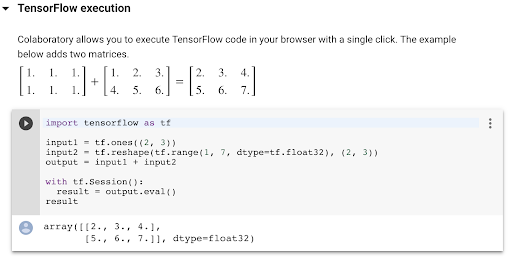
Figure X shows shows how Google Collaboratory, one of many tools to interact with Jupyter notebooks, leverages the power of Jupyter extensions for custom interaction and presentation.

Google Collaboratory uses Jupyter extensions to customize Jupyter for their users. The run/play icon to the left of the code cell is created using extensions. This is not present in the standard Jupyter software. TensorFlow is a library for creating Machine Learning experiments in Python.

Google Collaboratory uses Jupyter extensions to customize Jupyter for their users. The run/play icon to the left of the code cell is created using extensions. This is not present in the standard Jupyter software. TensorFlow is a library for creating Machine Learning experiments in Python.

The set of extensions for Jupyter is constantly evolving. Educators are exploring new and interesting methods of using notebooks in pedagogy. While the list of current extensions is far too long to list, you can interactively experience some of the most useful extensions through this live Binder notebook (Binder is described in detail in the following chapter). This live notebook demonstrates the following:

  • Turning on line numbers in code cells (makes it easier to refer to a line of code)
  • Code folding extension (hide code blocks to help focus attention)
  • Locked and frozen cells extension (prevent changes to cells)
  • An extension for a better user interface for error messages
  • A “turtle” extension (draws in a canvas in the notebook)
  • Block-based programming extension

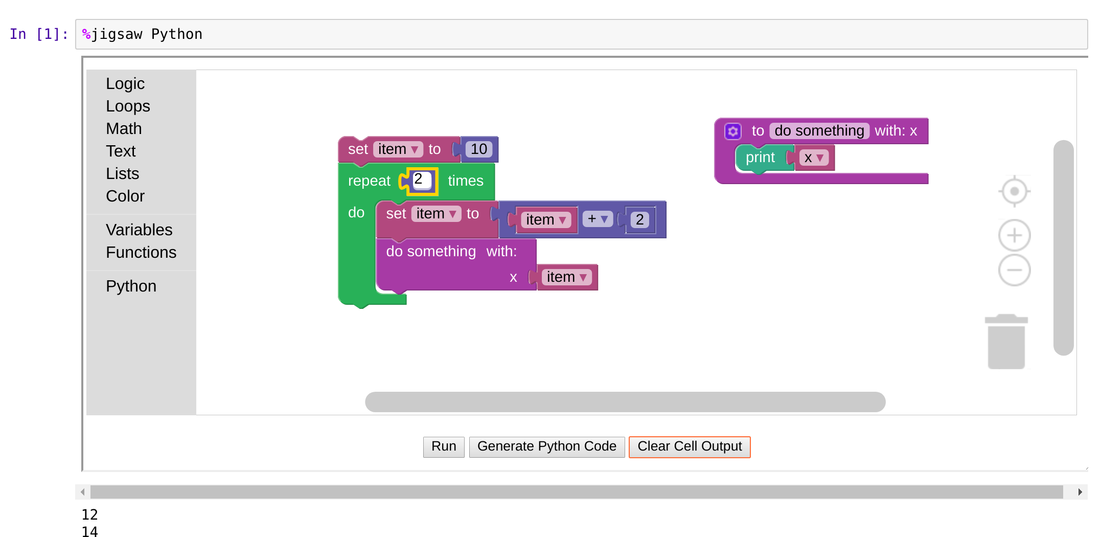
The block-based programming extension (called Jigsaw) allows users to program using drag-and-drop blocks of code that can be integrated with other cells in a Jupyter Notebook (see figure). The advantages (and disadvantages) of blocked-based languages are active research topics in computer education research (see, for example, Mark Guzdial’s excellent Computing Education Research Blog, specifically those posts on block-based languages).

Example of incorporating Jigsaw, a block-based extension, in a Jupyter Notebook. The extension allows the user to assemble code blocks that can then be translated into Python or Java, and executed.

Example of incorporating Jigsaw, a block-based extension, in a Jupyter Notebook. The extension allows the user to assemble code blocks that can then be translated into Python or Java, and executed.

5.4 Tips and tricks

5.4.1 Reminders

If you are using a single notebook as a standalone exercise in a traditional class (i.e., this is the only computational component of your class), then it is helpful to have a few cells at the top of that notebook that reviews how to navigate through the notebook and how to insert cells, etc.

5.4.2 Feedback

How do we get feedback from students in an interactive session to see if students have completed an exercise?

A low tech solution is to give students sticky notes of different colors, one meaning “finished” and one meaning “need help”, that they can stick on the back of their computers. The instructor can then quickly look up to take a survey of the state of the class and decide how to proceed.

Projecting Slack or a similar chat group on a screen and having student copy-paste solutions (provided they are short functions) is a nice way to let everyone in the class see one another’s solutions. A positive aspect of having multiple student solutions projected is that it can show the variety of ways to solve a problem. This gives an opportunity to talk about the readability of solutions and their efficiency. A downside is that in a large class, the sheer volume of posts can make it overwhelming. Instead polling can be used to aggregate student answers and provide some form of feedback to the instructor. Nbgrader or travis-CI can also be options here, requiring students to submit completed code where it is assessed automatically. These will however require more setup and can take some time to complete.

5.4.3 Explaining each cell

Consider moving the comments for a code block into a markdown cell either directly above or below the code cell. Comments in a markdown cell often read much better and give you more flexibility in discussing or describing the code. However, short comments in a block of code can still be useful.

5.4.4 How to structure code cells

How much code should you put in a cell? You will develop your own style of writing noteooks with experience. Typically, you will want to keep the number of lines low so that it is easy to follow, and you can have useful comments above the cell. However, we recommend putting code that “goes together as a meaningful unit” into a single cell. For example, if you have lines of code that are highly dependent on each other, then you might want to put them together. As an example, consider two lines of code: one that opens a file, and the second that reads the data from the file. It is probably a good idea to put those into the same cell so that they are always executed together. Otherwise, the student may encounter errors if they execute cells independently a second time (e.g., there are no more data).

Specifically, messing up the dependencies between cells is where most of the confusion using notebooks comes from with new users. For example, if you change a variable’s name (without restarting the notebook), then the following code cells may continue to use the old variable’s name (and value). Later, when running the notebook again, the notebook may fail in unexpected ways because the old variable no longer exists. This is sometimes referred to as “the hidden state problem.” This is an open research problem, and researchers are exploring various possible solutions. For example, trying searching the internet for “jupyter dependency graph” or “jupyter dataflow notebook.”

Pro Tip

You can easily split a cell into two parts at the cursor using the keystroke CONTROL + SHIFT + -. You can also merge multiple cells with SHIFT + m. Both of these are also available from the menu under Edit.

On the other hand, it is often a useful idea to separate lines of code where you want to provide the student a place to interactively add cells, and examine the state at that particular point in the process. Asking probing questions in a Socratic method is a very useful technique for engaging the reader and encouraging them to become more than a reader. Students do not naturally know to insert cells and explore items in a notebook. You will need to explicitly teach this skill. In fact, teaching students how to effectively weave code into their own notebook stories is an important component of teaching with notebooks.

5.4.5 Custom styling

New notebook creators often try to centrally manage the formatting of headings, equations, and other textual items. For example, rather than using a standard markdown heading, a creator may over-design the headings by using HTML styles. This may create two problems:

  1. The rendering of the notebook markdown may change and your formatted HTML header may not maintain the same look over time.

  2. Headers created using markdown can be used by notebook tools, such as automatically creating a Table of Contents.

Our recommendation is to resist the desire to customize the styling and simply use the default representations. If you want to do customization (for example if you want to color certain cells) you can use CSS.

5.4.6 Length of notebooks

Notebook authors sometimes make the notebooks very long with many topics and sections. Notebook sections and cells are currently not easily reused in a copy/paste sense for mixing intra-notebook content. Until this functionality is available, we recommend that authors make short, self-contained notebooks around short topics. This allows other notebooks authors to mix and match notebooks to create curriculum.

5.5 Gotchas

5.5.1 Programming language \(\neq\) Jupyter

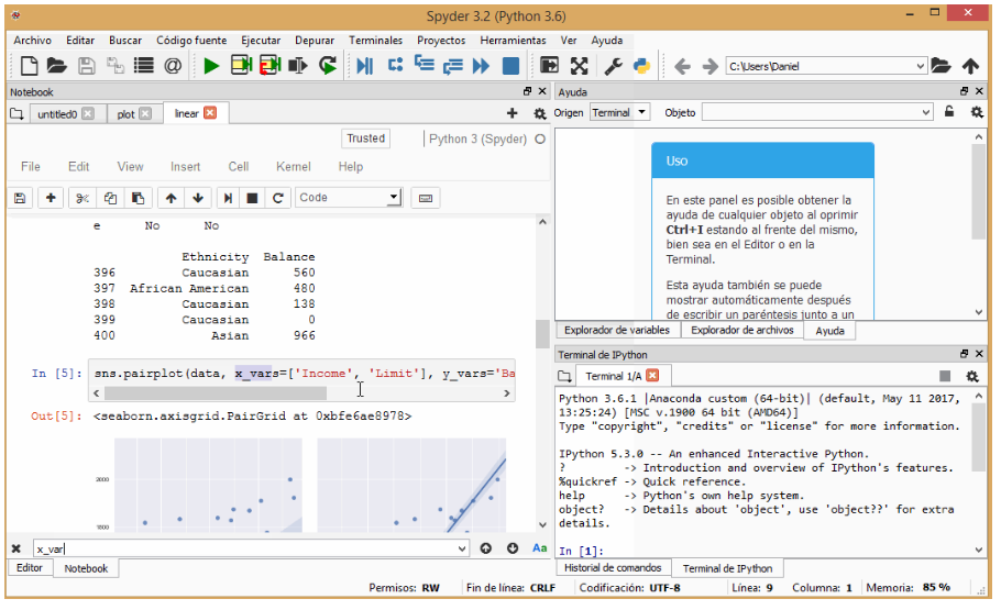
Teaching a class entirely with Jupyter can give the sense to students that this is the way all computational exploration is done. In particular, students can be confused into thinking that programming requires the notebook, instead of understanding that a notebook is just one way to interact with a particular language. This point should be made clear periodically. A good way to reinforce this is to show how to take a function that has been developed and debugged in a notebook and cut-paste it into a script (such as a file ending in .py for Python) and then import it into the notebook to regain that functionality. Also, the Integrated Development Environment (IDE), Spyder, has a plugin (https://github.com/spyder-ide/spyder-notebook) that allows notebooks to be displayed alongside Python scripts and a python terminal which can be useful for showing this dichotomy.
Jupyter notebook displayed in a window pane inside Spyder.

Jupyter notebook displayed in a window pane inside Spyder.

5.5.2 Restart, restart, restart…

Often, students may need to stop a computation, and this can be accomplished by pressing the “Interrupt” button in the toolbar. However, students should also be made aware of how to restart the kernel in a notebook, and what this means. There are several instances when students might need to do this. Sometimes students write code that can go into an infinite loop. The visual cues that notebooks give in this case are subtle, and students may not realize this and don’t understand why the notebook is non-responsive. In live-coding situations, it can be useful to demonstrate this to students and show them how to restart the kernel and carry on.

A second instance of where restarting a kernel might be needed is due to how the notebook stores the state of the computation. We like to think that, since the notebook is laid out in a linear fashion, that the state will always reflect what would happen if the notebook was run from the start up to that point. However, it is common to work in a notebook out of order, for instance if students ask a question about some previous example. If the variable has been changed in subsequent cells, then its value might not reflect what you expect when you rerun a cell earlier in the notebook. Restarting the kernel is sometimes the only solution.

5.5.3 Notebook hygiene

Many gotchas can be mitigated by developing notebooks that will be robust to incremental and non-linear execution. The main principle is to minimize side-effects of executing a cell and manifests itself somewhat differently in different languages; our suggestions here will be relevant to Python and may need to be adapted for other languages. Notebooks should generally be able to execute sequentially, such as via “restart kernel and run all cells”. (An exception is when a notebook is intentionally incomplete for the purpose of live coding or student exercises, see nbgrader or the exercise estnations for more elegant ways to handle this.) Variable mutation is the most common way in which a notebook may malfunction when executing cells in a non-linear way (e.g., in response to student questions or when comparing and contrasting different methodologies). Sometimes this mutation is incidental, through dummy variables that were not meant to have significance outside the scope of the cell in which they are used. Their scope can be limited by placing them in a function, even if that function is only called once. Redefinition of functions can often be avoided by parameterizing the desired functionality as would typically be done if designing a library (though this may be a distracting software design for novice programmers). Function definitions should have little or no dependency on variables from their enclosing scope. When modifying cells for demos and formative assessments during class, it is useful to either copy the cell or modify/execute such that a conforming implementation remains present when moving on to other cells where it may be used. Additionally, you can minimize these issues by grouping code in a single cell that should always be executed sequentially, because code within a cell will always be sequential.